> ## Documentation Index
> Fetch the complete documentation index at: https://cockroachlabs.mintlify.site/llms.txt
> Use this file to discover all available pages before exploring further.
# Spatial Indexes
export const InternalLink = ({version, path = "", children, ...props}) => {
let detectedVersion = version || "stable";
if (typeof window !== 'undefined' && !version) {
const match = window.location.pathname.match(/\/docs\/([^/]+)/);
if (match) {
detectedVersion = match[1];
}
}
const normalizedPath = path.startsWith("/") ? path.slice(1) : path;
return
{children}
;
};
This page describes CockroachDB's support for indexing spatial data, including:
* What spatial indexes are
* How they work
* How to create and tune spatial indexes in CockroachDB
CockroachDB does not support indexing geospatial types in default primary keys, nor in
unique secondary indexes.
## What is a spatial index?
At a high level, a spatial index is just like any other index. Its purpose is to improve your database's performance by helping SQL locate data without having to look through every row of a table.
Spatial indexes store information about spatial objects, but they are used for the same tasks as any other index type, i.e.,
* Fast filtering of lists of shapes based on spatial predicate functions such as `ST_Contains`.
* Speeding up joins that involve spatial data columns.
Spatial indexes differ from other types of indexes as follows:
* They are specialized to operate on 2-dimensional `GEOMETRY` and `GEOGRAPHY` data types. They are stored by CockroachDB as a special type of GIN index. For specifics, see [Details](#details).
* If needed, they can be tuned to store looser or tighter coverings of the shapes being indexed, depending on the needs of your application. Tighter coverings are more expensive to generate, store, and update, but can perform better in some cases because they return fewer false positives during the initial index lookup. Tighter coverings can also lead to worse performance due to more rows in the index, and more scans at the storage layer. That's why we recommend that most users should not need to change the default settings. For more information, see [Tuning spatial indexes](#tuning-spatial-indexes).
## How CockroachDB's spatial indexing works
There are two main approaches to building geospatial indexes:
* One approach is to "divide the objects" by inserting the objects into a tree (usually an [R-tree](https://wikipedia.org/wiki/R-tree)) whose shape depends on the data being indexed. This is the approach taken by [PostGIS](https://postgis.net/).
* The other approach is to "divide the space" by creating a decomposition of the space being indexed into buckets of various sizes.
CockroachDB takes the "divide the space" approach to spatial indexing. This is necessary to preserve CockroachDB's ability to scale horizontally by adding nodes to a running cluster.
CockroachDB uses the "divide the space" approach for the following reasons:
* It's easy to scale horizontally.
* It requires no balancing operations, unlike [R-tree indexes](https://wikipedia.org/wiki/R-tree).
* Inserts under this approach require no locking.
* Bulk ingest is simpler to implement than under other approaches.
* It allows advanced users to make a per-object tradeoff between index size and false positives during index creation. (See [Tuning spatial indexes](#tuning-spatial-indexes).)
Whichever approach to indexing is used, when an object is indexed, a "covering" shape (i.e., a bounding box) is constructed that completely encompasses the indexed object. Index queries work by looking for containment or intersection between the covering shape for the query object and the indexed covering shapes. This retrieves false positives but no false negatives.
### Details
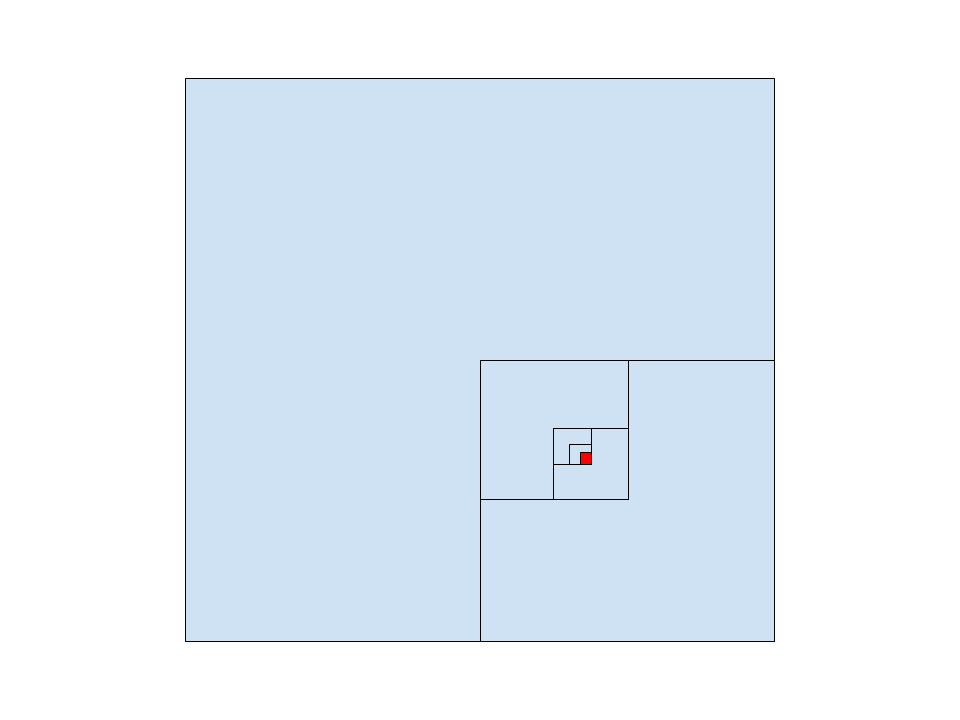
Under the hood, CockroachDB uses the [S2 geometry library](https://s2geometry.io/) to divide the space being indexed into a [quadtree](https://wikipedia.org/wiki/Quadtree) data structure with a set number of levels and a data-independent shape. Each node in the quadtree (really, [S2 cell](https://s2geometry.io/devguide/s2cell_hierarchy)) represents some part of the indexed space and is divided once horizontally and once vertically to produce 4 child cells in the next level. The following image shows visually how a location (marked in red) is represented using levels of a quadtree:
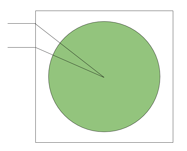
 Visually, you can think of the S2 library as enclosing a sphere in a cube. We map from points on each face of the cube to points on the face of the sphere. As you can see in the following 2-dimensional picture, there is a projection that occurs in this mapping: the lines entering from the left mark points on the cube face, and are "refracted" by the material of the cube face before touching the surface of the sphere. This projection reduces the distortion that would occur if the points on the cube face were projected straight onto the sphere.
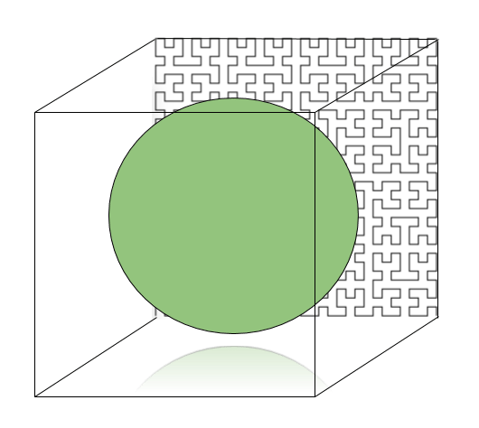
 Next, let's look at a 3-dimensional image that shows the cube and sphere more clearly. Each cube face is mapped to the quadtree data structure mentioned, and each node in the quadtree is numbered using a [Hilbert space-filling curve](https://wikipedia.org/wiki/Hilbert_curve) which preserves locality of reference. In the following image, you can imagine the points of the Hilbert curve on the rear face of the cube being projected onto the sphere in the center. The use of a space-filling curve means that two shapes that are near each other on the sphere are very likely to be near each other on the line that makes up the Hilbert curve. This is good for performance.
 When you index a spatial object, a covering is computed using some number of the cells in the quadtree. The number of covering cells can vary per indexed object by passing special arguments to `CREATE INDEX` that tell CockroachDB how many levels of S2 cells to use. The leaf nodes of the S2 quadtree are at level 30, and for `GEOGRAPHY` measure 1cm across the Earth's surface. By default, `GEOGRAPHY` indexes use up to level 30, and get this level of precision. We also use S2 cell coverings in a slightly different way for `GEOMETRY` indexes. The precision you get there is the bounding length of the `GEOMETRY` index divided by 4^30. For more information, see [Tuning spatial indexes](#tuning-spatial-indexes).
CockroachDB stores spatial indexes as a special type of GIN index. The spatial index maps from a location, which is a square cell in the quadtree, to one or more shapes whose coverings include that location. Since a location can be used in the covering for multiple shapes, and each shape can have multiple locations in its covering, there is a many-to-many relationship between locations and shapes.
## Tuning spatial indexes
The information in this section is for advanced users doing performance optimization. Most users should not need to
change the default settings. Without careful testing, you can get worse performance by changing the default settings.
When an object is indexed, a "covering" shape (e.g., a bounding box) is constructed that completely encompasses the indexed object. Index queries work by looking for containment or intersection between the covering shape for the query object and the indexed covering shapes. This retrieves false positives but no false negatives.
This leads to a tradeoff when creating spatial indexes. The number of cells used to represent an object in the index is tunable: fewer cells use less space, but create a looser covering. A looser covering retrieves a larger amount of positives from the index, which is expensive because the exact answer computation that's run after the index query can be expensive. However, at some point the benefits of retrieving fewer false positives is outweighed by how long it takes to scan a large index.
Another consideration is that the larger index created for a tighter covering is more expensive to scan and to update, especially for write-heavy workloads.
We strongly recommend leaving your spatial indexes at the default settings unless you can take at least the following steps:
1. Verify the coverings that will be generated meet your accuracy expectations by using the `st_s2covering` function as shown in [View an object's S2 covering](#view-an-object’s-s2-covering).
2. Do extensive performance tests to make sure the indexes that use the non-default coverings actually provide a performance benefit.
### Visualize index coverings
In what follows we will visualize how index coverings change as we change the `s2_max_cells` parameter, which determines how much work CockroachDB will perform to find a tight covering of a shape.
We will generate coverings for the following geometry object, which describes a shape whose vertices land on some small cities in the Northeastern US:
```text theme={"theme":{"light":"catppuccin-mocha","dark":"catppuccin-mocha"}}
'SRID=4326;LINESTRING(-76.4955 42.4405, -75.6608 41.4102,-73.5422 41.052, -73.929 41.707, -76.4955 42.4405)'
```
The animated following image shows the S2 coverings that are generated as we increase the `s2_max_cells` parameter from the 1 to 30 (minimum to maximum):
When you index a spatial object, a covering is computed using some number of the cells in the quadtree. The number of covering cells can vary per indexed object by passing special arguments to `CREATE INDEX` that tell CockroachDB how many levels of S2 cells to use. The leaf nodes of the S2 quadtree are at level 30, and for `GEOGRAPHY` measure 1cm across the Earth's surface. By default, `GEOGRAPHY` indexes use up to level 30, and get this level of precision. We also use S2 cell coverings in a slightly different way for `GEOMETRY` indexes. The precision you get there is the bounding length of the `GEOMETRY` index divided by 4^30. For more information, see [Tuning spatial indexes](#tuning-spatial-indexes).
CockroachDB stores spatial indexes as a special type of GIN index. The spatial index maps from a location, which is a square cell in the quadtree, to one or more shapes whose coverings include that location. Since a location can be used in the covering for multiple shapes, and each shape can have multiple locations in its covering, there is a many-to-many relationship between locations and shapes.
## Tuning spatial indexes
The information in this section is for advanced users doing performance optimization. Most users should not need to
change the default settings. Without careful testing, you can get worse performance by changing the default settings.
When an object is indexed, a "covering" shape (e.g., a bounding box) is constructed that completely encompasses the indexed object. Index queries work by looking for containment or intersection between the covering shape for the query object and the indexed covering shapes. This retrieves false positives but no false negatives.
This leads to a tradeoff when creating spatial indexes. The number of cells used to represent an object in the index is tunable: fewer cells use less space, but create a looser covering. A looser covering retrieves a larger amount of positives from the index, which is expensive because the exact answer computation that's run after the index query can be expensive. However, at some point the benefits of retrieving fewer false positives is outweighed by how long it takes to scan a large index.
Another consideration is that the larger index created for a tighter covering is more expensive to scan and to update, especially for write-heavy workloads.
We strongly recommend leaving your spatial indexes at the default settings unless you can take at least the following steps:
1. Verify the coverings that will be generated meet your accuracy expectations by using the `st_s2covering` function as shown in [View an object's S2 covering](#view-an-object’s-s2-covering).
2. Do extensive performance tests to make sure the indexes that use the non-default coverings actually provide a performance benefit.
### Visualize index coverings
In what follows we will visualize how index coverings change as we change the `s2_max_cells` parameter, which determines how much work CockroachDB will perform to find a tight covering of a shape.
We will generate coverings for the following geometry object, which describes a shape whose vertices land on some small cities in the Northeastern US:
```text theme={"theme":{"light":"catppuccin-mocha","dark":"catppuccin-mocha"}}
'SRID=4326;LINESTRING(-76.4955 42.4405, -75.6608 41.4102,-73.5422 41.052, -73.929 41.707, -76.4955 42.4405)'
```
The animated following image shows the S2 coverings that are generated as we increase the `s2_max_cells` parameter from the 1 to 30 (minimum to maximum):
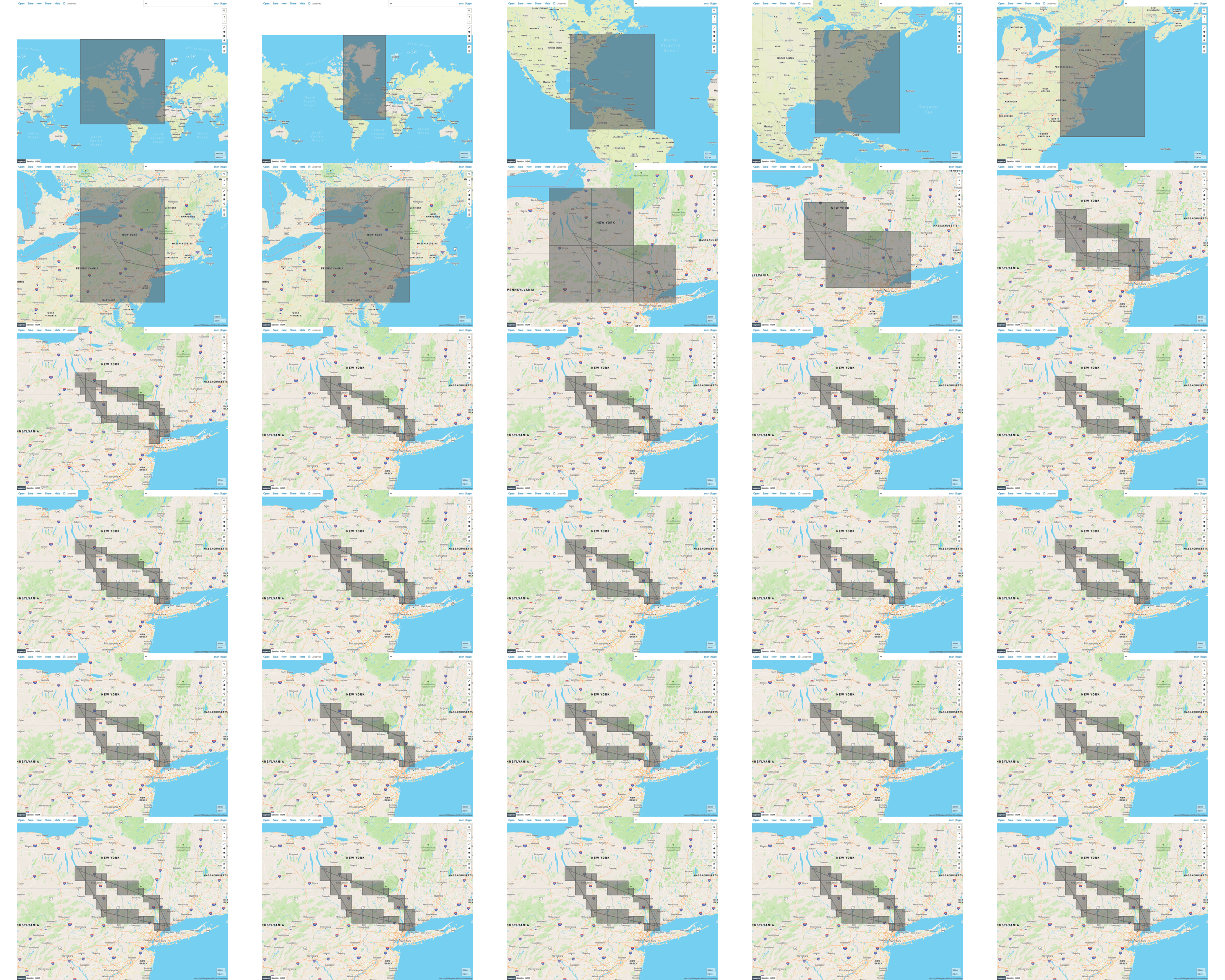
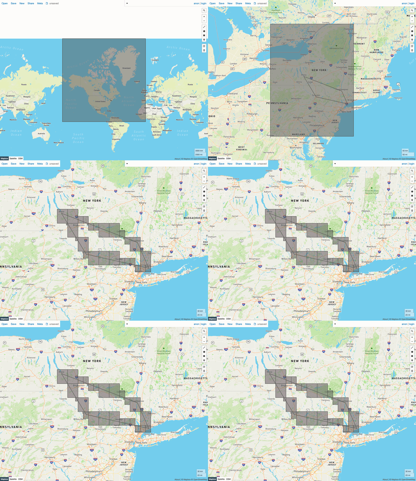 Here are the same images presented in a grid. You can see that as we turn up the `s2_max_cells` parameter, more work is done by CockroachDB to discover a tighter and tighter covering (that is, a covering using more and smaller cells). The covering for this particular shape reaches a reasonable level of accuracy when `s2_max_cells` reaches 10, and stops improving much past 12.
 ### Index tuning parameters
The following parameters are supported by both `CREATE INDEX` and the built-in function `st_s2covering`. The latter is useful for seeing what kinds of coverings would be generated by an index with various tuning parameters if you were to create it. For an example showing how to use these parameters with `st_s2covering`, see [View an object's S2 covering](#view-an-object’s-s2-covering).
If a shape falls outside the bounding coordinates determined by the following `geometry_*` settings, there will be a
performance loss in that such shapes may not be eliminated by the index lookup, but the database will still return the
correct answers.
| Option | Default value | Description |
| ------------------ | --------------------------------------------- | -------------------------------------------------------------------------------------------------------------------------------------------------------------------------------------------------------------------------------------------------------------------------------------------------------------------------------------------------------------------------------------------------------------------------------------------------------------------------------------------------- |
| `s2\_level\_mod` | 1 | `s2\_max\_level` must be divisible by `s2\_level\_mod`. `s2\_level\_mod` must be between `1` and `3`. |
| `s2\_max\_level` | 30 | The maximum level of S2 cell used in the covering. Allowed values: 1-30. Setting it to less than the default means that CockroachDB will be forced to generate coverings using larger cells. |
| `s2\_max\_cells` | 4 | The maximum number of S2 cells used in the covering. Provides a limit on how much work is done exploring the possible coverings. Allowed values: 1-30. You may want to use higher values for odd-shaped regions such as skinny rectangles. |
| `geometry\_min\_x` | Derived from SRID bounds, else `-(1 << 31)` | Minimum X-value of the spatial reference system for the object(s) being covered. This only needs to be set if the default bounds of the SRID are too large/small for the given data, or SRID = 0 and you wish to use a smaller range (unfortunately this is currently not exposed, but is viewable on \< [https://epsg](https://epsg). io/3857). By default, SRID = 0 assumes `[-min int32, max int32]` ranges. |
| `geometry\_max\_x` | Derived from SRID bounds, else `(1 << 31) -1` | Maximum X-value of the spatial reference system for the object(s) being covered. This only needs to be set if you are using a custom SRID. |
| `geometry\_min\_y` | Derived from SRID bounds, else `-(1 << 31)` | Minimum Y-value of the spatial reference system for the object(s) being covered. This only needs to be set if you are using a custom SRID. |
| `geometry\_max\_y` | Derived from SRID bounds, else `(1 << 31) -1` | Maximum Y-value of the spatial reference system for the object(s) being covered. This only needs to be set if you are using a custom SRID. |
## Examples
### View an object's S2 covering
Here is an example showing how to pass the [spatial index tuning parameters](#index-tuning-parameters) to `st_s2covering`. It generates [GeoJSON](https://geojson.org/) output showing both a shape and the S2 covering that would be generated for that shape in your index, if you passed the same parameters to `CREATE INDEX`. You can paste this output into [geojson.io](http://geojson.io/) to see what it looks like.
```sql theme={"theme":{"light":"catppuccin-mocha","dark":"catppuccin-mocha"}}
CREATE TABLE tmp_viz (id INT8, geom GEOMETRY);
INSERT INTO tmp_viz (id, geom)
VALUES (1, st_geomfromtext('LINESTRING(-76.8261 42.1727, -75.6608 41.4102,-73.5422 41.052, -73.929 41.707, -76.8261 42.1727)'));
INSERT INTO tmp_viz (id, geom)
VALUES (2, st_s2covering(st_geomfromtext('LINESTRING(-76.8261 42.1727, -75.6608 41.4102,-73.5422 41.052, -73.929 41.707, -76.8261 42.1727)'), 's2_max_cells=20,s2_max_level=12,s2_level_mod=3,geometry_min_x=-180,geometry_max_x=180,geometry_min_y=-180,geometry_max_y=180'));
SELECT ST_AsGeoJSON(st_collect(geom)) FROM tmp_viz;
```
```json theme={"theme":{"light":"catppuccin-mocha","dark":"catppuccin-mocha"}}
{
"type": "GeometryCollection",
"geometries": [
{
"type": "LineString",
"coordinates": [
[-76.8261, 42.1727],
[-75.6608, 41.4102],
[-73.5422, 41.052],
[-73.929, 41.707],
[-76.8261, 42.1727]
]
},
{
"type": "MultiPolygon",
"coordinates": [
[
[
[-76.904296875, 42.099609375],
[-76.81640625, 42.099609375],
[-76.81640625, 42.1875],
[-76.904296875, 42.1875],
[-76.904296875, 42.099609375]
]
],
[
[
[-76.81640625, 42.099609375],
[-76.728515625, 42.099609375],
[-76.728515625, 42.1875],
[-76.81640625, 42.1875],
[-76.81640625, 42.099609375]
]
],
[
[
[-76.728515625, 42.099609375],
[-76.640625, 42.099609375],
[-76.640625, 42.1875],
[-76.728515625, 42.1875],
[-76.728515625, 42.099609375]
]
],
[
[
[-76.728515625, 42.01171875],
[-76.640625, 42.01171875],
[-76.640625, 42.099609375],
[-76.728515625, 42.099609375],
[-76.728515625, 42.01171875]
]
],
[
[
[-76.640625, 41.484375],
[-75.9375, 41.484375],
[-75.9375, 42.1875],
[-76.640625, 42.1875],
[-76.640625, 41.484375]
]
],
[
[
[-74.53125, 40.78125],
[-73.828125, 40.78125],
[-73.828125, 41.484375],
[-74.53125, 41.484375],
[-74.53125, 40.78125]
]
],
[
[
[-73.828125, 40.78125],
[-73.125, 40.78125],
[-73.125, 41.484375],
[-73.828125, 41.484375],
[-73.828125, 40.78125]
]
],
[
[
[-73.828125, 41.484375],
[-73.740234375, 41.484375],
[-73.740234375, 41.572265625],
[-73.828125, 41.572265625],
[-73.828125, 41.484375]
]
],
[
[
[-74.53125, 41.484375],
[-73.828125, 41.484375],
[-73.828125, 42.1875],
[-74.53125, 42.1875],
[-74.53125, 41.484375]
]
],
[
[
[-75.234375, 41.484375],
[-74.53125, 41.484375],
[-74.53125, 42.1875],
[-75.234375, 42.1875],
[-75.234375, 41.484375]
]
],
[
[
[-75.234375, 40.78125],
[-74.53125, 40.78125],
[-74.53125, 41.484375],
[-75.234375, 41.484375],
[-75.234375, 40.78125]
]
],
[
[
[-75.322265625, 41.30859375],
[-75.234375, 41.30859375],
[-75.234375, 41.396484375],
[-75.322265625, 41.396484375],
[-75.322265625, 41.30859375]
]
],
[
[
[-75.41015625, 41.30859375],
[-75.322265625, 41.30859375],
[-75.322265625, 41.396484375],
[-75.41015625, 41.396484375],
[-75.41015625, 41.30859375]
]
],
[
[
[-75.5859375, 41.396484375],
[-75.498046875, 41.396484375],
[-75.498046875, 41.484375],
[-75.5859375, 41.484375],
[-75.5859375, 41.396484375]
]
],
[
[
[-75.5859375, 41.30859375],
[-75.498046875, 41.30859375],
[-75.498046875, 41.396484375],
[-75.5859375, 41.396484375],
[-75.5859375, 41.30859375]
]
],
[
[
[-75.498046875, 41.30859375],
[-75.41015625, 41.30859375],
[-75.41015625, 41.396484375],
[-75.498046875, 41.396484375],
[-75.498046875, 41.30859375]
]
],
[
[
[-75.673828125, 41.396484375],
[-75.5859375, 41.396484375],
[-75.5859375, 41.484375],
[-75.673828125, 41.484375],
[-75.673828125, 41.396484375]
]
],
[
[
[-75.76171875, 41.396484375],
[-75.673828125, 41.396484375],
[-75.673828125, 41.484375],
[-75.76171875, 41.484375],
[-75.76171875, 41.396484375]
]
],
[
[
[-75.849609375, 41.396484375],
[-75.76171875, 41.396484375],
[-75.76171875, 41.484375],
[-75.849609375, 41.484375],
[-75.849609375, 41.396484375]
]
],
[
[
[-75.9375, 41.484375],
[-75.234375, 41.484375],
[-75.234375, 42.1875],
[-75.9375, 42.1875],
[-75.9375, 41.484375]
]
]
]
}
]
}
```
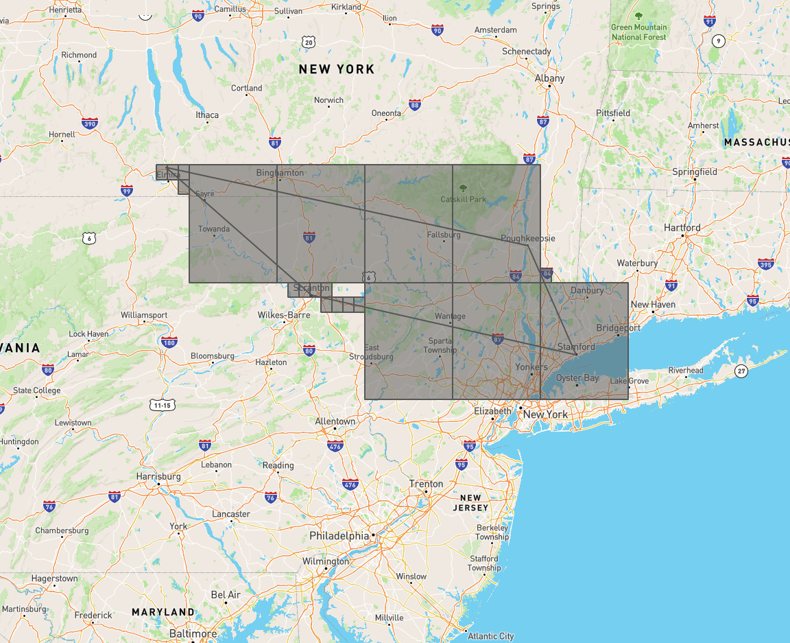
When you paste the JSON output into [geojson.io](http://geojson.io/), it generates the following picture, which shows both the `LINESTRING` and its S2 covering based on the options you passed to `st_s2covering`.
### Index tuning parameters
The following parameters are supported by both `CREATE INDEX` and the built-in function `st_s2covering`. The latter is useful for seeing what kinds of coverings would be generated by an index with various tuning parameters if you were to create it. For an example showing how to use these parameters with `st_s2covering`, see [View an object's S2 covering](#view-an-object’s-s2-covering).
If a shape falls outside the bounding coordinates determined by the following `geometry_*` settings, there will be a
performance loss in that such shapes may not be eliminated by the index lookup, but the database will still return the
correct answers.
| Option | Default value | Description |
| ------------------ | --------------------------------------------- | -------------------------------------------------------------------------------------------------------------------------------------------------------------------------------------------------------------------------------------------------------------------------------------------------------------------------------------------------------------------------------------------------------------------------------------------------------------------------------------------------- |
| `s2\_level\_mod` | 1 | `s2\_max\_level` must be divisible by `s2\_level\_mod`. `s2\_level\_mod` must be between `1` and `3`. |
| `s2\_max\_level` | 30 | The maximum level of S2 cell used in the covering. Allowed values: 1-30. Setting it to less than the default means that CockroachDB will be forced to generate coverings using larger cells. |
| `s2\_max\_cells` | 4 | The maximum number of S2 cells used in the covering. Provides a limit on how much work is done exploring the possible coverings. Allowed values: 1-30. You may want to use higher values for odd-shaped regions such as skinny rectangles. |
| `geometry\_min\_x` | Derived from SRID bounds, else `-(1 << 31)` | Minimum X-value of the spatial reference system for the object(s) being covered. This only needs to be set if the default bounds of the SRID are too large/small for the given data, or SRID = 0 and you wish to use a smaller range (unfortunately this is currently not exposed, but is viewable on \< [https://epsg](https://epsg). io/3857). By default, SRID = 0 assumes `[-min int32, max int32]` ranges. |
| `geometry\_max\_x` | Derived from SRID bounds, else `(1 << 31) -1` | Maximum X-value of the spatial reference system for the object(s) being covered. This only needs to be set if you are using a custom SRID. |
| `geometry\_min\_y` | Derived from SRID bounds, else `-(1 << 31)` | Minimum Y-value of the spatial reference system for the object(s) being covered. This only needs to be set if you are using a custom SRID. |
| `geometry\_max\_y` | Derived from SRID bounds, else `(1 << 31) -1` | Maximum Y-value of the spatial reference system for the object(s) being covered. This only needs to be set if you are using a custom SRID. |
## Examples
### View an object's S2 covering
Here is an example showing how to pass the [spatial index tuning parameters](#index-tuning-parameters) to `st_s2covering`. It generates [GeoJSON](https://geojson.org/) output showing both a shape and the S2 covering that would be generated for that shape in your index, if you passed the same parameters to `CREATE INDEX`. You can paste this output into [geojson.io](http://geojson.io/) to see what it looks like.
```sql theme={"theme":{"light":"catppuccin-mocha","dark":"catppuccin-mocha"}}
CREATE TABLE tmp_viz (id INT8, geom GEOMETRY);
INSERT INTO tmp_viz (id, geom)
VALUES (1, st_geomfromtext('LINESTRING(-76.8261 42.1727, -75.6608 41.4102,-73.5422 41.052, -73.929 41.707, -76.8261 42.1727)'));
INSERT INTO tmp_viz (id, geom)
VALUES (2, st_s2covering(st_geomfromtext('LINESTRING(-76.8261 42.1727, -75.6608 41.4102,-73.5422 41.052, -73.929 41.707, -76.8261 42.1727)'), 's2_max_cells=20,s2_max_level=12,s2_level_mod=3,geometry_min_x=-180,geometry_max_x=180,geometry_min_y=-180,geometry_max_y=180'));
SELECT ST_AsGeoJSON(st_collect(geom)) FROM tmp_viz;
```
```json theme={"theme":{"light":"catppuccin-mocha","dark":"catppuccin-mocha"}}
{
"type": "GeometryCollection",
"geometries": [
{
"type": "LineString",
"coordinates": [
[-76.8261, 42.1727],
[-75.6608, 41.4102],
[-73.5422, 41.052],
[-73.929, 41.707],
[-76.8261, 42.1727]
]
},
{
"type": "MultiPolygon",
"coordinates": [
[
[
[-76.904296875, 42.099609375],
[-76.81640625, 42.099609375],
[-76.81640625, 42.1875],
[-76.904296875, 42.1875],
[-76.904296875, 42.099609375]
]
],
[
[
[-76.81640625, 42.099609375],
[-76.728515625, 42.099609375],
[-76.728515625, 42.1875],
[-76.81640625, 42.1875],
[-76.81640625, 42.099609375]
]
],
[
[
[-76.728515625, 42.099609375],
[-76.640625, 42.099609375],
[-76.640625, 42.1875],
[-76.728515625, 42.1875],
[-76.728515625, 42.099609375]
]
],
[
[
[-76.728515625, 42.01171875],
[-76.640625, 42.01171875],
[-76.640625, 42.099609375],
[-76.728515625, 42.099609375],
[-76.728515625, 42.01171875]
]
],
[
[
[-76.640625, 41.484375],
[-75.9375, 41.484375],
[-75.9375, 42.1875],
[-76.640625, 42.1875],
[-76.640625, 41.484375]
]
],
[
[
[-74.53125, 40.78125],
[-73.828125, 40.78125],
[-73.828125, 41.484375],
[-74.53125, 41.484375],
[-74.53125, 40.78125]
]
],
[
[
[-73.828125, 40.78125],
[-73.125, 40.78125],
[-73.125, 41.484375],
[-73.828125, 41.484375],
[-73.828125, 40.78125]
]
],
[
[
[-73.828125, 41.484375],
[-73.740234375, 41.484375],
[-73.740234375, 41.572265625],
[-73.828125, 41.572265625],
[-73.828125, 41.484375]
]
],
[
[
[-74.53125, 41.484375],
[-73.828125, 41.484375],
[-73.828125, 42.1875],
[-74.53125, 42.1875],
[-74.53125, 41.484375]
]
],
[
[
[-75.234375, 41.484375],
[-74.53125, 41.484375],
[-74.53125, 42.1875],
[-75.234375, 42.1875],
[-75.234375, 41.484375]
]
],
[
[
[-75.234375, 40.78125],
[-74.53125, 40.78125],
[-74.53125, 41.484375],
[-75.234375, 41.484375],
[-75.234375, 40.78125]
]
],
[
[
[-75.322265625, 41.30859375],
[-75.234375, 41.30859375],
[-75.234375, 41.396484375],
[-75.322265625, 41.396484375],
[-75.322265625, 41.30859375]
]
],
[
[
[-75.41015625, 41.30859375],
[-75.322265625, 41.30859375],
[-75.322265625, 41.396484375],
[-75.41015625, 41.396484375],
[-75.41015625, 41.30859375]
]
],
[
[
[-75.5859375, 41.396484375],
[-75.498046875, 41.396484375],
[-75.498046875, 41.484375],
[-75.5859375, 41.484375],
[-75.5859375, 41.396484375]
]
],
[
[
[-75.5859375, 41.30859375],
[-75.498046875, 41.30859375],
[-75.498046875, 41.396484375],
[-75.5859375, 41.396484375],
[-75.5859375, 41.30859375]
]
],
[
[
[-75.498046875, 41.30859375],
[-75.41015625, 41.30859375],
[-75.41015625, 41.396484375],
[-75.498046875, 41.396484375],
[-75.498046875, 41.30859375]
]
],
[
[
[-75.673828125, 41.396484375],
[-75.5859375, 41.396484375],
[-75.5859375, 41.484375],
[-75.673828125, 41.484375],
[-75.673828125, 41.396484375]
]
],
[
[
[-75.76171875, 41.396484375],
[-75.673828125, 41.396484375],
[-75.673828125, 41.484375],
[-75.76171875, 41.484375],
[-75.76171875, 41.396484375]
]
],
[
[
[-75.849609375, 41.396484375],
[-75.76171875, 41.396484375],
[-75.76171875, 41.484375],
[-75.849609375, 41.484375],
[-75.849609375, 41.396484375]
]
],
[
[
[-75.9375, 41.484375],
[-75.234375, 41.484375],
[-75.234375, 42.1875],
[-75.9375, 42.1875],
[-75.9375, 41.484375]
]
]
]
}
]
}
```
When you paste the JSON output into [geojson.io](http://geojson.io/), it generates the following picture, which shows both the `LINESTRING` and its S2 covering based on the options you passed to `st_s2covering`.
 ### Create a spatial index
The following example shows how to create a spatial index on a `GEOMETRY` object using the default settings:
```sql theme={"theme":{"light":"catppuccin-mocha","dark":"catppuccin-mocha"}}
CREATE INDEX geom_idx_1 ON some_spatial_table USING GIST(geom);
```
### Create a spatial index with non-default tuning parameters
The following examples show how to create spatial indexes with non-default settings for some of the [spatial index tuning parameters](#index-tuning-parameters):
```sql theme={"theme":{"light":"catppuccin-mocha","dark":"catppuccin-mocha"}}
CREATE INDEX geom_idx_1 ON geo_table1 USING GIST(geom) WITH (s2_level_mod=3);
CREATE INDEX geom_idx_2 ON geo_table2 USING GIST(geom) WITH (geometry_min_x=0, s2_max_level=15)
CREATE INDEX geom_idx_3 ON geo_table3 USING GIST(geom) WITH (s2_max_level=10)
CREATE INDEX geom_idx_4 ON geo_table4 USING GIST(geom) WITH (geometry_min_x=0, s2_max_level=15);
```
### Create spatial indexes during table definition
This example shows how to create a table with spatial indexes on `GEOMETRY` and `GEOGRAPHY` types that use non-default settings for some of the [spatial index tuning parameters](#index-tuning-parameters):
```sql theme={"theme":{"light":"catppuccin-mocha","dark":"catppuccin-mocha"}}
CREATE TABLE public.geo_table (
id INT8 NOT NULL,
geog GEOGRAPHY(GEOMETRY,4326) NULL,
geom GEOMETRY(GEOMETRY,3857) NULL,
CONSTRAINT "primary" PRIMARY KEY (id ASC),
INVERTED INDEX geom_idx_1 (geom) WITH (s2_max_level=15, geometry_min_x=0),
INVERTED INDEX geom_idx_2 (geom) WITH (geometry_min_x=0),
INVERTED INDEX geom_idx_3 (geom) WITH (s2_max_level=10),
INVERTED INDEX geom_idx_4 (geom),
INVERTED INDEX geog_idx_1 (geog) WITH (s2_level_mod=2),
INVERTED INDEX geog_idx_2 (geog),
FAMILY fam_0_geog (geog),
FAMILY fam_1_geom (geom),
FAMILY fam_2_id (id)
)
```
### Create a spatial index that uses all of the tuning parameters
This example shows how to set all of the [spatial index tuning parameters](#index-tuning-parameters) at the same time. It is extremely unlikely you will ever need to set all of the options at once; this example is being provided to show the syntax.
```sql theme={"theme":{"light":"catppuccin-mocha","dark":"catppuccin-mocha"}}
CREATE INDEX geom_idx
ON some_spatial_table USING GIST(geom)
WITH (s2_max_cells = 20, s2_max_level = 12, s2_level_mod = 3,
geometry_min_x = -180, geometry_max_x = 180,
geometry_min_y = -180, geometry_max_y = 180);
```
As noted, most users should not change the default settings. There is a risk that you will get worse performance by
changing the default settings.
### Create a spatial index on a `GEOGRAPHY` object
The following example shows how to create a spatial index on a `GEOGRAPHY` object using the default settings:
```sql theme={"theme":{"light":"catppuccin-mocha","dark":"catppuccin-mocha"}}
CREATE INDEX geog_idx_3 ON geo_table USING GIST(geog);
```
## See also
* GIN Indexes
* [S2 Geometry Library](https://s2geometry.io/)
* Indexes
* Spatial Data Overview
* Spatial tutorial
* Export Spatial Data
* Spatial and GIS Glossary of Terms
* Spatial functions
* Migrate from Shapefiles
* Migrate from GeoJSON
* Migrate from GeoPackage
* Migrate from OpenStreetMap
* [Introducing Distributed Spatial Data in CockroachDB](https://www.cockroachlabs.com/blog/spatial-data) (blog post)
* Using GeoServer with CockroachDB
### Create a spatial index
The following example shows how to create a spatial index on a `GEOMETRY` object using the default settings:
```sql theme={"theme":{"light":"catppuccin-mocha","dark":"catppuccin-mocha"}}
CREATE INDEX geom_idx_1 ON some_spatial_table USING GIST(geom);
```
### Create a spatial index with non-default tuning parameters
The following examples show how to create spatial indexes with non-default settings for some of the [spatial index tuning parameters](#index-tuning-parameters):
```sql theme={"theme":{"light":"catppuccin-mocha","dark":"catppuccin-mocha"}}
CREATE INDEX geom_idx_1 ON geo_table1 USING GIST(geom) WITH (s2_level_mod=3);
CREATE INDEX geom_idx_2 ON geo_table2 USING GIST(geom) WITH (geometry_min_x=0, s2_max_level=15)
CREATE INDEX geom_idx_3 ON geo_table3 USING GIST(geom) WITH (s2_max_level=10)
CREATE INDEX geom_idx_4 ON geo_table4 USING GIST(geom) WITH (geometry_min_x=0, s2_max_level=15);
```
### Create spatial indexes during table definition
This example shows how to create a table with spatial indexes on `GEOMETRY` and `GEOGRAPHY` types that use non-default settings for some of the [spatial index tuning parameters](#index-tuning-parameters):
```sql theme={"theme":{"light":"catppuccin-mocha","dark":"catppuccin-mocha"}}
CREATE TABLE public.geo_table (
id INT8 NOT NULL,
geog GEOGRAPHY(GEOMETRY,4326) NULL,
geom GEOMETRY(GEOMETRY,3857) NULL,
CONSTRAINT "primary" PRIMARY KEY (id ASC),
INVERTED INDEX geom_idx_1 (geom) WITH (s2_max_level=15, geometry_min_x=0),
INVERTED INDEX geom_idx_2 (geom) WITH (geometry_min_x=0),
INVERTED INDEX geom_idx_3 (geom) WITH (s2_max_level=10),
INVERTED INDEX geom_idx_4 (geom),
INVERTED INDEX geog_idx_1 (geog) WITH (s2_level_mod=2),
INVERTED INDEX geog_idx_2 (geog),
FAMILY fam_0_geog (geog),
FAMILY fam_1_geom (geom),
FAMILY fam_2_id (id)
)
```
### Create a spatial index that uses all of the tuning parameters
This example shows how to set all of the [spatial index tuning parameters](#index-tuning-parameters) at the same time. It is extremely unlikely you will ever need to set all of the options at once; this example is being provided to show the syntax.
```sql theme={"theme":{"light":"catppuccin-mocha","dark":"catppuccin-mocha"}}
CREATE INDEX geom_idx
ON some_spatial_table USING GIST(geom)
WITH (s2_max_cells = 20, s2_max_level = 12, s2_level_mod = 3,
geometry_min_x = -180, geometry_max_x = 180,
geometry_min_y = -180, geometry_max_y = 180);
```
As noted, most users should not change the default settings. There is a risk that you will get worse performance by
changing the default settings.
### Create a spatial index on a `GEOGRAPHY` object
The following example shows how to create a spatial index on a `GEOGRAPHY` object using the default settings:
```sql theme={"theme":{"light":"catppuccin-mocha","dark":"catppuccin-mocha"}}
CREATE INDEX geog_idx_3 ON geo_table USING GIST(geog);
```
## See also
* GIN Indexes
* [S2 Geometry Library](https://s2geometry.io/)
* Indexes
* Spatial Data Overview
* Spatial tutorial
* Export Spatial Data
* Spatial and GIS Glossary of Terms
* Spatial functions
* Migrate from Shapefiles
* Migrate from GeoJSON
* Migrate from GeoPackage
* Migrate from OpenStreetMap
* [Introducing Distributed Spatial Data in CockroachDB](https://www.cockroachlabs.com/blog/spatial-data) (blog post)
* Using GeoServer with CockroachDB